
|
||||
The aim of this unit is to provide a measure of spatial awareness together with a brief introduction to Geographic Information Systems, GIS, and some of the techniques upon which it is founded.
We live in a 4-dimensional world. Human beings have always had to consider how things are arranged spatially in such a world and how they might change with time, whether it was palaeolithic hunters deciding how best to stalk their next meal or 20th Century planners deciding where to site a new supermarket. With population increase and industrialisation continuing to exert pressure on the land available it is more important than ever that information about spatial relationships and trends can be collected, stored and processed efficiently. Although such activities have been going on for hundreds of years the basic system involved is always the same.
Any system is essentially a dynamic entity which can receive inputs, process them in some way and produce outputs. In the past, systems dealing with information have been largely paper-based with someone's brain doing the processing in the middle. If the information is spatially-based in some way then we have the essence of a Geographical Information System.
The term Geographical may be regarded by some as being too disciplinary specific. It could easily be replaced by terms such as spatial, environmental, land etc. But the term Geographical is now in such widespread usage that it is here to stay.
The development of information technology (IT) has already had a profound effect on many aspects of life. Over the past decade or so the rapid advances in computing hardware have dramatically increased the potential for producing IT systems to effectively manage and process spatial information, which is invariably more complex than non-spatial information.
Many of the early computer-based Geographical Information Systems (in the rest of this guide the term GIS refers specifically to computer-based geographical information systems) have been relatively technical and only really accessible to people with a high level of computer literacy. The purpose of this Study Guide is to introduce you to a particular GIS called ArcView that has been designed specifically to make GIS accessible to a much wider audience.
You are advised to work steadily through the Guide although, depending upon your background, you may be able to skip through some sections relatively quickly. To help you consolidate your understanding there are Self-Assessment Questions (SAQs) for you to try with the answers in the back of the guide.
For most of the Guide you will need access to a computer with ArcView installed. However, before actually sitting down at the keyboard it is worth considering briefly how we have dealt with spatial information before the advent of GIS and some pointers to how GIS mirrors and modifies this approach. If you are a geographer or familiar with using maps you may want to go straight on to section 2, but if this is relatively new to you or your memory needs refreshing then work through this introductory section before you switch on the computer.
1.1.1 Features
Plate 1.1 shows a portion of landscape consisting of a number of features such as buildings, roads, fields etc.
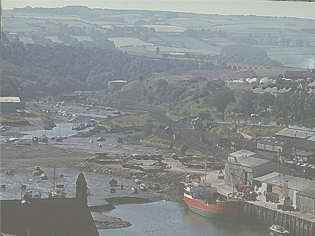
Plate 1 - Photo of Whitby, copyright (c) PJ Halls, 1975, Used with permission.
The traditional way of recording spatial information about this particular piece of landscape would be on a paper map of the type shown in Fig. 1.1.
Fig. 1.1. Map of Whitby
In essence, the map can give us three types of information about the features that make up the landscape:-
1) their spatial arrangement
2) their shape
3) their size
A map will always provide information on 1) about all of the features that it shows. However, depending upon their size and the scale of the map (see 1.1.2 below) some features may only be shown by a symbol (which tells us virtually nothing about their actual size and shape) at the appropriate place on the map. For example, in Fig. 1.1 the size and shape of the area of woodland is clearly shown but the bus station symbol tells us nothing about its shape or size, except that it must be a lot smaller than the woodland!
The meanings of the various symbols used are usually given in a key alongside the map. On the key of Ordnance Survey maps, similar types of features are grouped into categories or themes (e.g. roads and paths, boundaries, water features etc.). During the period BC (Before Computer!), if it was necessary to analyse the themes that make up a map, they could be drawn as a series of separate overlays to make the analysis easier, as shown in Fig. 1.2
Fig. 1.2. Schematic 3D diagram of map from Fig. 1.1
1.1.2 Scale
For a map to be as accurate as possible the sizes of features and distances between them should be in the same proportion as they are in the real world. This is done by drawing the map to scale. The number of times the real world distances are greater than the map distances gives the magnitude of the scale e.g. 1 cm on the map may represent 50000cm (i.e. half km) in the real world, hence the scale would be 1:50000 . Scale can also be represented as a scale bar (see Fig. 1.1).
When real world distances have been reduced to relatively small distances on the map it is known as a small scale map whereas when the real world distance is represented by quite large distances on a map it is known as a large scale map. Another way of considering this is that on a standard size of paper, say A4, a map covering the whole of England would be small scale whereas, on the same piece of paper, a map covering a few streets in a town would be large scale. The boundary between large and small scale is not officially defined but in the United Kingdom, in general, anything at 1:10000 or larger (e.g. 1:2500, 1:1250) is large scale and anything smaller than 1:10000 would be small scale.
SAQ 1. What is the scale of the map in Fig. 1.3?
Fig. 1.3 Road lengths in kilometers.
It also needs to be remembered that scale influences the accuracy with which location can be shown. Although cartographers (people who produce maps) always aim for accuracy in showing the location of one feature relative to another, the margin of error on the map associated with a feature's actual location on the ground is likely to increase as the scale of the map decreases. There are many reasons for this. Some are that cartographic conventions often result in, for example, a road of a particular classification always being drawn at a standard line width and that point features (e.g. windmills) are always drawn at a constant size. Sometimes features that, when represented at a small scale would overlay each other, are deliberately slightly displaced so that they are all visible, e.g. a road, railway and river co-existing in a steep-sided valley.
1.1.3 Co-ordinates
To use a map effectively it is important to have some means of identifying the location of a particular feature. When trying to indicate where something is, people often describe it in relationship to something else "up the road, turn left and it's just opposite the supermarket". This is all very well if you are always coming from the same location but if your starting point varies those instructions are not much use.
If you look at a model of the globe, you should observe vertical lines being drawn joining the North and South poles and a series of horizontal lines being drawn between these poles.
Fig. 1.4. Map of globe, showing latitude & longitude graticules
The vertical lines are lines of longitude and the horizontal lines are lines of latitude. The equator is the most famous latitude and is given the arbitrary value of zero. The North and South poles are given the arbitrary value of 90. So all locations between the equator and the poles have a value lying somewhere between 0 and 90. If you look at an atlas, you will observe that the southern most tip of Cornwall, in south-west England has a latitude of approximately 50. Cartographers call latitudes north of the equator, Northings (Guess what those south of the equator are called!).
Some time last century it was internationally agreed to give the value zero to the vertical line, or longitude that passes through Greenwich in London. Cartographers call Longitudes east of Greenwich, Eastings. (Guess what those west of Greenwich are called!). We will conveniently ignore for now what happens when you have got half way round the world.
Using a latitude value and a longitude value it is possible to uniquely locate any position on the globe. These lines do not, of course, actually exist on the earth, but over the centuries, cartographers have found them to be a convenient way of identifying locations.
However, it is often not very convenient to use these particular lines on large scale maps. In such circumstances, cartographers commonly use some form of grid system, tailored to the specific needs of a particular country.
For those of you who can remember drawing graphs at school, you will recall that the horizontal axis was often also called the 'x' axis and the vertical axis was often called the 'y' axis. Any point which had an x and y value could be located, or represented on the graph. In a similar way, imagine the outline of the UK drawn as a series of x,y values on a graph. Also imagine that the x,y value of 0,0 (which is equivalent to the origin of a graph) is in the Atlantic Ocean just off the Scilly Isles, which are located west of the Cornish mainland. Every location in the UK can now be given a unique x,y value, also known as a pair of coordinates.
This describes a simplified version of a special grid which the Ordnance Survey use for maps of the UK, and which they call the National Grid, (not to be confused with the other national grid which delivers electricity across the country!). In this grid, the UK is divided up into large squares of 100km x 100km (called, not surprisingly, 100km squares) and the origin of this coordinate system (i.e. the x,y cordinates 0,0) is indeed just west of the Scilly Isles. The x values increase moving eastwards to Kent and the y values increase moving northwards to the Shetland Isles. Pinching terminology used above, locations east of this origin are called Eastings and locations north of this origin are called Northings. So an x,y pair of coordinates can be identified for all intersections between the horizontal and vertical lines in the grid.
But how are features located that do not conveniently fall at these 100km grid intersections? This is resolved by further dividing each 100km grid square into 10km grid squares. In turn, each 10km grid square can be further divided into 1km grid squares, and so on. The extent to which you wish to continue such subdivision depends upon the accuracy at which you wish to represent the location of a point. This in turn will be influenced by whether you are using a large scale map (lots of detail) or a small scale map (not so much detail).
Consider first, just the Easting. The 100km line will be represented by a single digit. This will be 0 or 1 or 2 etc. Representing the horizontal (i.e. x ) value of the bottom left hand corner of the 100km grid square which contains the feature of interest. The 10km subdivisions of the 100km Easting will be represented by a second digit, the 1km subdivisions of the 10km Easting will be represented by a third digit and so on, with the 1m subdivisions represented by a sixth digit. A similar subdivision can be made for the Northing.
Fig. 1.5.
In such an example, the grid reference would therefore consist of twelve digits, the first six representing the Easting and the second six digits representing the Northing.
Such a grid reference can look uncomfortably indigestable and would only be used for very large scale maps. For, say the Ordnance Survey 1:250,000 maps, a grid reference expressed as eight digits, the first four for the Easting and the second four for the Northing be located. The eight figure grid reference for the church with a spire in Fig 1.6 is 54561782
Fig. 1.6.
Purely for completeness, though at the risk of adding some confusion, two alternative but related ways in which the Ordnance Survey express grid references should be noted, because it is often used on their paper maps. Rather than express a grid reference as e.g. 54561782 the Easting and Northing 100km digits are written first, and then followed by the 10km and subsequent digits for first the Eastings and then the 10km and subsequent digits for the Northings. So this grid reference would be written as 51/254798. A further variant is that the 100km squares are given a two letter code, so 51 is also known as TQ, giving a grid reference expressed as TQ254798. But computers are much happier dealing with an all-digit representation with a logical hiararchy from 100km, 10km, 1km etc. so we shall not consider the alternative representations any further.
Fig. 1.7
SAQ 2. Describe what is found at grid reference 48905094 in Fig. 1.7.
SAQ 3. Using Fig 1.7 to identify the grid lines in Fig. 1.1, what is the grid reference for Ruswarp Police Office in Fig 1.1. What is the grid reference for the pub (PH) in Fig. 1.7?
1.1.4 Representing height
Ignoring the 4th dimension (time) for the moment, we can say that a map, with length and width, is a 2-dimensional representation of a 3D world which in reality has not only length and width but also height. Therefore there needs to be some way of indicating how this 3rd dimension (height) varies. This can only be done if there is an agreed 'baseline' to measure the height from. On Ordnance Survey maps this is known as the vertical datum and is the mean sea level at Newlyn in Cornwall.
Height is represented on maps in a number of ways. The height of an individual point can be given as a spot height or, as the height of a triangulation pillar, which is a concrete post often situated on the top of a hill and from which the height of other points visible from the hill can be accurately measured (see Fig. 1.7). In fact, such trig. points are becoming increasingly redundant as it is now possible to measure very accurately the location (including height) of any point on the Earth using stereo photogrammetry and, increasingly, satellite technology. Many maps also have contour lines, each of which joins up all the points at the same height. The closer together the contours are the steeper the slope is. With practice, by studying the contours on the map you can get a good picture in your mind of the general 3-dimensional landform.
Fig. 1.8
SAQ 4. Briefly describe the landform shown on the map in Fig. 1.8.
1.1.5 Map Layouts
The layout of a map can vary but if it is to be of maximum use to the person studying it there are certain essential components that must be present. These would include whatever themes were appropriate for that map together with the necessary grid for co-ordinates, scale, key, north arrow and, of course, a title!
We have seen how a paper map contains information about the size, shape and spatial relationships of features in the real world. However, there may be other information about a feature or features that we need to know. For example, a traffic planner might need to know the number of vehicles per hour passing along a particular road or someone in business might need to know how many sales she or he was making in a particular town. This type of information (known as thematic information) would not be shown on a general-purpose map and the person requiring it would have to obtain it from another source and, if they wanted to represent it spatially in some way, draw a special map to do so.
In addition, there may be topographical information (which is about specific locations that could be shown on a map) that cannot appear on a particular map because of its scale. For example, an ecologist might need to know the number, distribution and type of tree species growing in a particular wood, which itself can only be shown as an area of green on the map.
A GIS provides an opportunity to store both these kinds of non-spatial information (also often called descriptive or attribute information, as well as the spatial information contained within the map itself, in a single system. In current GISs these two types of information (spatial and non-spatial) are often stored in two separate databases (essentially, the term used for storing data in a computer in a particular structured way). However, the two databases are linked or joined together so that, for example, the characteristics of a line in the spatial database can be identified as representing a road and that it is a motorway; a point represents a church, and the church has a tower, etc. etc. An analogy might be the way we mentally link information with particular features on a map. The term georelational is sometimes used to describe the connection between a spatial database and the corresponding attributes in the attribute database.
However, a GIS is not merely a means of storing and displaying information. Increasingly, its strengths lie in its processing or analytical capabilities. This might involve integrating (e.g. overlaying) data from different themes to find a solution to some form of planning problem e.g. integrating data from road, urban area and wildlife habitat themes to identify possible routes for a by-pass. Also, a GIS can incorporate the influence of the 4th dimension, time, very easily into the analysis. This might involve comparing the same types of data for a particular area over a period of time to establish any trends e.g. how fast scrub is invading an area of grassland.
For this reason, GIS is becoming increasingly important to a growing number of activities and professions. These include people involved with any aspects of land use (e.g. planning, agriculture, forestry, nature conservation), human population studies (e.g. research into the geographical distribution of particular diseases like so-called 'cancer clusters'), commerce, environmental monitoring and management etc. etc.
By now you should have some very general impressions of what a GIS is and what its potentials are. Before passing on to more details about the specific characteristics of ArcView, this section concludes with what is not exactly a precise definition of GIS but does emphasise its very wide appeal and potential!
"GIS is a sort of culture, born of a multi-disciplinary content, where every actor brings their skill, their point of view and their own GIS definition."
David Rhind (Director General of the Ordnance Survey)
Chapter One of Principles of Geographical Information Systems for Land Resources Assessment, P. A. Burrough, Oxford University Press.
Graphics Multimedia Virtual Environments Visualisation Contents