
|
||||
The aim of this unit is to introduce the more powerful characteristics of GIS, such as statistical and overlay analysis, which collectively, in the context of a GIS are often termed Spatial Analysis. These techniques go beyond those introduced in UNIT 2, which are little more than techniques of display and presentation. This then presents you with an Introductory Analysis Assignment.
Analysis is about selecting those parts of your data which are relevant to the task in hand, and using them to attempt to find answers to questions. Analysis with a GIS, often termed spatial analysis, unlike other Information Systems, has the added dimension of 'space' or geography. This combination of descriptive attributes on various phenomena, e.g. a person's age, the type of road etc, together with information on e.g. where a person lives or the location of a road, permits a variety of locational questions to be asked such as where are ..., show me where ..., how far is ..., what is next to ..., what is this ..., are there any ... near this ..., ... In addition, where information relating to time is also available, these may also include such questions as how long will it take to get from ... to ... and how long before ... reaches ...
It is this ability to perform spatial analysis which marks GIS as being different from drawing tools, Computer Aided Design (CAD) tools, and mapping systems. Although GIS can be used to produce maps - and often to a standard of quality equal to any 'mapping' tool - it is the very combination of analysis with display, and data input and management, capability that gives GIS its particular distinctive properties. Put succinctly, in a GIS, display is usually regarded as a means to an end rather than the end in itself.
Using a GIS, the same information may be investigated in more than one way, using different spatial areas. For example, census returns might be analysed for the whole of the UK in order to determine the overall age: sex ratio of a population. Alternatively, the data may be dis-aggregated into separate counties, or even smaller areas such as Wards and Enumeration Districts perhaps to determine whether adequate school capacity is provided for the numbers of children in different areas, or to target the budget for community support services to communities comprising a high proportion of elderly people. Spatial Analysis, therefore, is about addressing the where component of information in addition to the what, when, and how much, which are identified as attributes of the 'where'..
Spatial analysis provides facilities for calculating a range of statistics for any of the attributes, e.g. area of polygons, length of arcs or perimeter of polygons as well as any of the e.g. census variables that you may have associated with e.g. a suite of polygons. You can also query your data to e.g. select and display only that data where roads represent motorways or census areas have 20% of the households owning two cars.
One of the particular distinctive characteristics of a GIS is the ability to overlay areas, rather like drawing areas on transparent paper and placing one on top of the other on an OHP to visually determine where phenomena on each of the transparencies overlap. For example, one layer may contain information of soils and soil boundaries, the other on crops and field boundaries. By overlaying the two maps, it is possible to observe the coincidence of crops with given soil types. One particularly useful overlay analysis available in ArcView is known as intersect. This makes it possible to identify where phenomena meet or cross. You will use this technique in the assignment later in this Unit.
Applications of spatial analysis, using GIS, include route planning (for example, the AutoRoute product or the AA's Routefinder), market analysis, insurance risk assessment, environmental impact assessments, emergency service dispatch and control ... and GIS is used by workers in disciplines as diverse as Social Policy and Ecology, Civil Engineering and Anthropology, Marketing and Politics!
ArcView provides the means to undertake a range of overlay analytical tasks. It should be noted, however, that the software does not attempt to fully replicate the functionality GIS software such as Arc/Info, which is also produced by ESRI, the additional functionality can be added to ArcView using Avenue, which is an additional product, which can be used to provide customised extensions.
Using a GIS, not only can the result of an overlay analysis be visually produced, but the result may itself be saved as a completely new dataset - itself then available to be used as a component of further analysis. For example, the results of one analysis may generate a zone of influence - the area affected by the release of a toxic gas perhaps from a factory chimney. This could be saved as a new theme and overlaid with e.g. the area of a housing estate to identify what areas, given various weather conditions, might be adversely affected, and so on. Finally, a spatial, statistical query could be constructed to identify the names of the residents that are affected, for ensuring that all have been safely evacuated, and to assist in establishing the provision of emergency accommodation pending the dispersion of the pollutant. There are no real limits to the extent of this process of deriving new datasets from the combination or interaction of one spatial dataset upon another, nor need the results necessarily be graphics, despite the use of geographic information during the computation process.
As noted in Unit 1 the real world is infinitely complex and we therefore need to use a much simpler representation or abstraction of reality. This abstraction is, in traditional cartographic terms, often seen as modelling reality either as points, lines or areas. It could therefore be argued that working with a GIS is always a modelling activity. For the purposes of this tutorial, however, the term model will be confined to refer to the active representations of processes which are intended to facilitate the understanding of that process and / or its interactions. This modelling concept is illustrated in Fig 1.
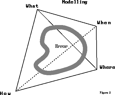
FIG 1
We have been displaying geographical information in terms of lines and areas, polygons. Some of these have, of course, a relationship with similar objects, with which they share a common boundary or maybe overlap. This spatial relationship between objects is termed the topology or the spatial topology. Some GIS make use of these relationships internally and store appropriate information that supports rapid access to information using these relationships - and also to avoid storing shared information, such as the co-ordinates that define a boundary between two adjacent polygons, more than once. GIS which build and maintain topology in this way are termed Topological GIS. It is this topological structure than enables many analyses to be performed. If the primary objective was merely to produce maps, then such a detailed structure would not be necessary. The term spaghetti structure is sometimes used to imply a minimalist ordering of the spatial data when only map production is required. ArcView does not, in fact use topology, but it can readily import data from Arc/Info which is topologically structured, as will be explained in the assignment later.
All analysis should also include an assessment of the reliability of solutions provided in answer to the question - the error rate. Some errors may be inherent in the data, due to sample size or distribution, accuracy of recording, frequency of re-processing, etc. Errors may also result from the application of a particular technique upon data that does not meet some minimum standard of quality. There may have been assumptions made about information not collected, or deemed to have little impact on the outcome of the investigation. It has been known for bad answers to have been produced as a result of using the wrong data! Some of these implications of data quality and fitness for purpose will be discussed in a later unit of this tutorial. Fig 2 offers a visual summary of these various inter-relationships of Analysis.
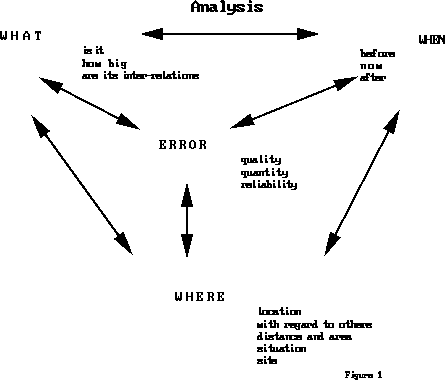
FIG 2
The inherent display facilities of a GIS, coupled with the speed of modern computers, make it an attractive tool for exploration forms of analysis, using the graphical display as a visualisation tool; a means to illustrate the results of the analysis or exploration. In this context, the term visualisation is used to describe not just the visual display but also the suite of mental processes you are using to achieve that display. For example, your analysis is frequently used to explore a number of what if ... scenarios potential alternative actions, or to visualise how a process operates in order to better understand side effects or components. An analogy could be the use of simulators used by trainee aircraft pilots. Similarly a GIS could be used by e.g. a town planner to explore the consequences of a proposed new road or housing estate.
The relative ease with visual images can now be displayed on modern computers, with easy-to-use software, can seduce the unwary into a false reliance upon material of a dubious nature. In computing circles there is a catch phrase, "garbage in, garbage out" - GIGO for short. With the use of GIS a very pretty, and appealing, map may readily be produced ... but which may have less meaning than many of the statistics bandied around by politicians seeking (re-)election. It is essential that every GIS user remain alert to the quality limitations of the data being used and the consequent implications for the quality of any analytic results, otherwise you may find yourself victim to "garbage in - pretty (meaningless) map out!"
There are many more techniques of spatial analysis than can be introduced in this tutorial course. Since some, perhaps many, of these may represent very new ways of thinking, this unit will gently explore some basic techniques and later modules will take these further, together with some more advanced procedures, and will also provide some ideas for further reading, for those who desire to learn more.
You will be using data, generously provided by Bartholomew, which will be used to create themes representing urban areas, rivers and administrative boundaries for Nottinghamshire and the surrounding area.
in the area to the bottom left. This is the query request and should be similar to Fig 4.
Query Builder form and you will be returned to the Theme Properties form.
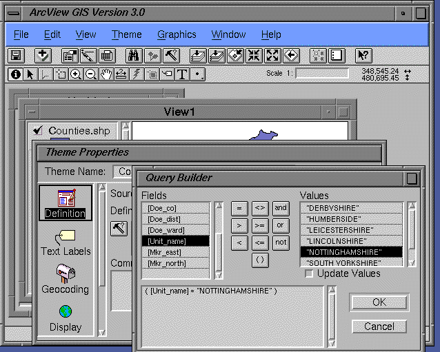
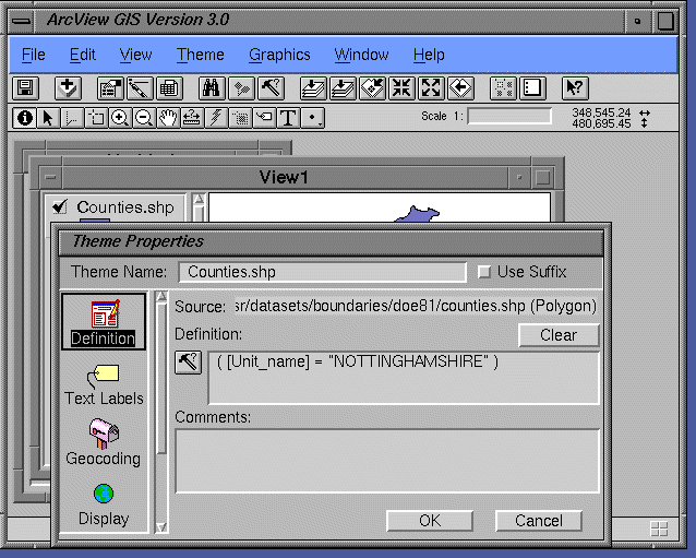 FIG 5
FIG 5 Note that, when you enable display of this data, it will appear as a small 'island' in a 'sea of nothing'. This is because the viewing area currently remains for the whole of the boundaries area but only a small part of this has been selected.
This theme contains details of rivers, major and minor, small streams and drainage channels, aqueducts and reservoir dams, in addition to canals. There are various classifications of each of these major features in addition. We only require the canals so it will be necessary, therefore, to use the Query Builder to refine the dataset for this exercise in order to have a theme which simply represents canals.
You now need to extract the canals from the Bartholomew drainage data. The different drainage features are classified using a field called Obs_acc_no. , Further, the 'canal' data required is divided up into a range of discrete features so that several values of obs_acc_no will be required. Only those categories likely to appear within the area of interest (Nottinghamshire) will be selected. These are (together with their Bartholomew explanations):
| Obs_acc_no value | Represents |
|---|---|
| 135641 | Canal class 'A' |
| 135642 | Canal class 'B' |
| 135643 | Canal class 'C' |
| 138682 | Canal tunnel |
This will select those records meeting the range of values specified.
([Obs_acc_no] >= 135641) and ([Obs_acc_no] <= 135643) or ([Obs_acc_no]="138682)"
This requires:
The display we now have, with the urban areas overlaying the county outline, gives an immediate visual impression, but not a quantitative evaluation.
Although ArcView, in itself, does not build spatial topology, it can make use of spatial topology that exists in feature source data imported from topology-based systems. The Bartholomew data is such as this, having been created by, and stored within Arc/Info, yet accessed directly with ArcView. Using Arc/Info, the area and perimeter of polygon data (areas) are automatically calculated and stored for every polygon, in the feature attribute table. This means that it is not necessary to calculate the area of the county of Nottinghamshire, rather, merely to examine the relevant field in the Nottinghamshire table.
Question 1: What is the area of Nottinghamshire? Note it down.
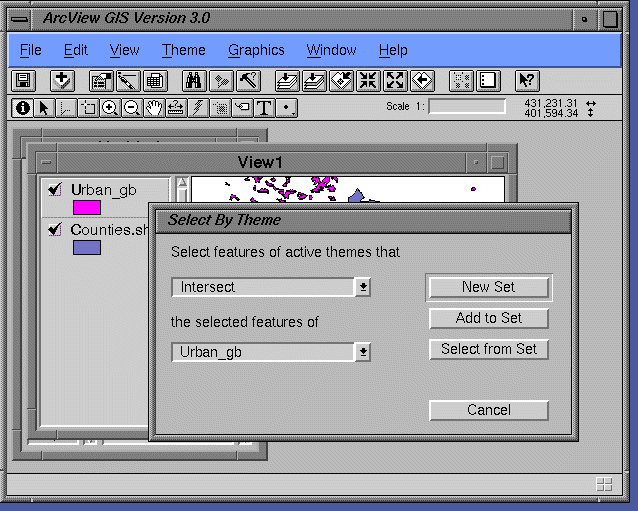
The Urban Areas Theme, as currently displayed, represents all the urban areas, not just those in Nottinghamshire! In order to extract just those areas of interest, a spatial overlay selection must be performed. The tool that will be used here, Intersect, will use the outline boundary of Nottinghamshire to select those objects in the Urban Areas Theme which lie within, or cross, this boundary. Clearly, doing it this way may introduce an over-estimation of the sum of the urban areas since it may include some space outside the Nottinghamshire boundary. This over-estimation will, in fact, be less than the under-estimation which would result from using only those areas contained wholly within the boundary - and excluding those which cross. In the interests of simplicity this error will be deemed acceptable at this time. A more accurate, but more complex, procedure will be introduced in a later unit.
Urban Area : (County Area - Urban Area)
Question 3: : What is the ratio, expressed arithmetically? Note it down.
To achieve this it is necessary to perform similar steps as above, but this time using all three datasets. Given that the urban areas of Nottinghamshire are a currently selected subset, use can be made of this by extracting this into a new theme, comprising just these records. So a completely new theme will be created as a result of performing a spatial overlay operation on two existing themes.
Select Intersect and Urban_gb.shp from the Window menu and click the New Set button.
(Note: Shapefiles are Arcview's internal method of storing spatial data.)
This requires you to use the summary statistics procedure, as used above to determine the sum of the urban areas of Nottinghamshire: this would be much easier (and more accurate) than repeating the earlier measurement procedure, from Unit 2, to measure the lengths of canal within the urban area boundaries.
The analytical tasks are now complete. Finish off by using the presentation skills learned in Unit 2, to create a layout, suitable for printing, which displays the county of Nottinghamshire with the Urban areas and the canals overlaid. The canals selected as passing through the urban areas should be distinguishable from the rest of the canal system.
With the completion of this unit, you should now be familiar with the following techniques:
Question 1: The area of the county of Nottinghamshire is 2,166,049,536.0 sq metres.
Question 2: The total of the urban areas that fall partially or totally within Nottinghamshire is 220,085,810 sq metres.
Question 3: The ratio of urban to rural Nottinghamshire is 2166049536 : 220085810.
Question 4: The length of canal selected is 74278.232 metres.
Suggestions for further reading
Chapters Five and Six of Principles of Geographical Information Systems for Land Resources Assessment, P. A. Burrough, 1986, Oxford University Press.
A classification of software components commonly used in geographic information systems, Jack Dangermond, 1990, in Introductory readings in Geographic Information Systems, Donna J. Peuquet and Duane F. Marble (eds), Taylor and Francis.
GIS versus CAD versus DBMS: what are the differences?, David J. Cowen, 1990, in Introductory readings in Geographic Information Systems, Donna J. Peuquet and Duane F. Marble (eds), Taylor and Francis.
Graphics Multimedia Virtual Environments Visualisation Contents