Editorial

Abstract

Introduction

The Projection Pursuit

RADVIZ

Parallel Coordinates

User Interaction

Finding Outliers

Conclusions

References

Appendix A - Datasets

Appendix B

Case Studies Index

3. The RADVIZ Approach to Visualisation}

Like the previous approach, the RADVIZ method (Ankerst et al., 1996) maps a set of m-dimensional points onto two dimensional space. However, in this case the mapping is nonlinear. To explain the RADVIZ approach, it is helpful to imaging a physical situation. Suppose m points are arranged to be equally spaced around the circumference of the unit circle. Call these points S₁ to S_m. Now suppose a set of m springs are fixed at one end to each of these points, and that all of the springs are attached to the other end to a puck, as in figure 7.

Figure 7: The Physical System Basis for RADVIZ

Finally, assume the stiffness constant (in terms of Hooke's law) of the jth string is x_ij for one of the data points i. If the puck is released and allowed to reach an equilibrium position, the coordinates of this position, (u_i, v_i)^T say, are the projection in two dimensional space of the point (x_i1, ..., x_im)^T in m-dimensional space. This, if (u_i, v_i)^T is computed for i = 1 ... n, and these points are plotted, a visualisation of the m-dimensional data set in two dimensions is achieved.

To discover more about the projection from R^m -> R², consider the forces acting on the puck. For a given spring, the force acting on the puck is the product of the vector spring extension and the scalar stiffness constant. The resultant force acting on the puck for all m springs will be the sum of these individual forces. When the puck is in equilibrium there are no resultant forces acting on it and this sum will be zero. Denoting the position vectors of S₁ to S_m by S₁ to S_m, and putting u_i = (u_i, v_i)^T we have

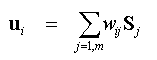
which may be solved for u_i by

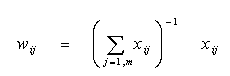
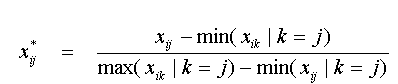
Thus, for each case i, u_i is simply a weighted mean of the S_j's whose weights are the m variables for case i normalised to sum to one. Note that this normalisation operation makes the mapping from R^m -> R² nonlinear.

Viewing the projection in this explicit form allows several of its properties to be deduced. First, assuming that the x_ij values are all non-negative, each u_i lies within the convex hull of the points S₁ to S_m,. Due to the regular spacing of these points, this convex hull will be an m-sided regular polygon. Note that if some of the x_ij values are negative this property need not hold, but that often each variable is re-scaled to avoid negative values. Two typical methods of doing this are the local metric (L-metric) rescaling, in which the minimum and maximum values of x_ij for each j are respectively mapped onto zero and one respectively:

and the global metric (G-metric), in which the rescaling is applied to the data set as a whole, rather than on a variable by variable basis:

in each case, the rescaled x_ij values will all lie in the interval [0,1].

The weighted centroid interpretation of the projection also allows some other properties to become apparent. If, for a given i, the values of x_ij are constant, u_i will be the zero vector. This is a rather strange property, since it implies that observations in which all variables take on a very high constant value (once re-scaled) will be projected onto the same point as observations in which all variables take on a very low constant value. More generally, it suggested that observations which take on very similar values for re-scaled data will be mapped into regions close to the origin.

A RADVIZ projection for the census data is shown in figure 8. The result is superficially similar to the maximised MNND projection pursuit, showing a circular cluster of points and identifying outliers around this.

Figure 8: A RADVIZ Projection of the Census Data

For general data sets this property could lead to difficulties in interpreting the plots, but it is particularly useful when considering compositional geographical data. Suppose the population of a geographical region is classified into m categories, for example, those aged under 18, those aged 18 to 65 and those aged over 65. Another example would be voting data for an electoral ward where the categories are the parties which each constituent voted for. A compositional data set is one in which each of the variables represents the proportion (or percentage) of each category for each area. Numerically, the most notable property of such data is that for each case the variables sum to 1 (or 100 if percentages are used). This constraint suggests that the only way that all m variables can be equal is when they all take the value 1/m. Note, however that even in this case, the fact that u_i = 0 does not imply that all proportions are equal. For example, if a pair of variables are represented by diametrically opposite points on the circle, and the proportions are 0.5 in each of these, then this will also give u_i = 0. Another aid to interpretation for compositional data is that if an area consists entirely of one category then the corresponding variable will take the value 1, while the others will take the value zero. This implies that u_i will lie on the vertex of the regular m-sided polygon corresponding to that category.

In the case m = 3 for compositional data the RADVIZ procedure produces the compositional triangular plot used for various purposes - notably by Dorling (1990) and Coombes et al. (1996) to illustrate voting patterns in Britain in a three-party system. If we were to extend the analysis to look at more than three parties (for example by considering the nationalist vote as a fourth option) then RADVIZ provides a natural extension of this concept. The main difficulty when moving beyond m = 3 for compositional data is that points on a RADVIZ plot no longer correspond uniquely to (x_i1, ... ,x_ij) for a given case, more than one composition can project onto the same u_i, as discussed above.

It is also interesting to note that for a given set of variables, there are several possible RADVIZ projections, since the $m$ initial m variables could be assigned to S₁ ... S_m in m! different ways. If we are mostly interested in identifying clusters and outliers, a number of possible projections will be essentially equivalent, since they will be identical up to a rotation or a mirror image. To see how many non-trivially different permutations there are, we need first to note that any permutation can be rotated m ways (i.e. rotation through 360/m degrees, by 2(260/m) degrees and so on up to (m - 1)(360/m) degrees, and of course the identity rotation through zero degrees), and so we need to divide the m! by m. We then note that any permutation can be reflected in two ways (i.e. mirror imaged or left alone) so the figure of (m - 1)! must be halved. Thus, if m is the number of variables, there are effectively (m - 1)! / 2 possible RADVIZ projections.

One way of deciding which of these should be used is to use an index, in a similar manner to projection pursuit in the previous section. In fact, the same indices could be used - for example maximising the variance of the u_i 's or using one of the nearest-neighbour distance based criteria. In this case, the optimisation is a discrete search over a finite number of possibilities, rather than a continuous multivariate optimisation problem as in projection pursuit. It should be noted that the number of options to be search increases very rapidly with m (worse than m²), and this has implications for computation. Clearly investigation into optimisation heuristics for this problem is necessary if it is to be applied in cases where m is very large.